How Are The Low And High Pass Filters For Dwt Chosen

Transform in numerical harmonic assay

An example of the 2D discrete wavelet transform that is used in JPEG2000. The original prototype is loftier-pass filtered, yielding the iii large images, each describing local changes in brightness (details) in the original image. It is then low-pass filtered and downscaled, yielding an approximation prototype; this epitome is high-pass filtered to produce the 3 smaller detail images, and low-laissez passer filtered to produce the terminal approximation epitome in the upper-left.^{[ clarification needed ]}

In numerical analysis and functional assay, a discrete wavelet transform (DWT) is any wavelet transform for which the wavelets are discretely sampled. As with other wavelet transforms, a primal advantage it has over Fourier transforms is temporal resolution: it captures both frequency and location information (location in time).

Examples [edit]

Haar wavelets [edit]

The first DWT was invented past Hungarian mathematician Alfréd Haar. For an input represented by a list of ${\displaystyle ii^{due north}}$ numbers, the Haar wavelet transform may be considered to pair up input values, storing the difference and passing the sum. This procedure is repeated recursively, pairing upwardly the sums to prove the side by side scale, which leads to ${\displaystyle 2^{n}-ane}$ differences and a final sum.

Daubechies wavelets [edit]

The most commonly used set of discrete wavelet transforms was formulated past the Belgian mathematician Ingrid Daubechies in 1988. This formulation is based on the use of recurrence relations to generate progressively finer detached samplings of an implicit female parent wavelet function; each resolution is twice that of the previous scale. In her seminal paper, Daubechies derives a family of wavelets, the first of which is the Haar wavelet. Interest in this field has exploded since then, and many variations of Daubechies' original wavelets were adult.^{[i] [2] [3]}

The dual-tree complex wavelet transform (DℂWT) [edit]

The dual-tree complex wavelet transform (ℂWT) is a relatively recent enhancement to the discrete wavelet transform (DWT), with of import additional backdrop: It is well-nigh shift invariant and directionally selective in ii and higher dimensions. Information technology achieves this with a redundancy cistron of merely ${\displaystyle 2^{d}}$ , substantially lower than the undecimated DWT. The multidimensional (M-D) dual-tree ℂWT is nonseparable just is based on a computationally efficient, separable filter depository financial institution (FB).^[iv]

Others [edit]

Other forms of detached wavelet transform include the LeGall-Tabatabai (LGT) five/3 wavelet developed by Didier Le Gall and Ali J. Tabatabai in 1988 (used in JPEG 2000 or JPEG XS ),^{[5] [half dozen] [7]} the Binomial QMF developed past Ali Naci Akansu in 1990,^[8] the fix division in hierarchical trees (SPIHT) algorithm developed by Amir Said with William A. Pearlman in 1996,^[9] the non- or undecimated wavelet transform (where downsampling is omitted), and the Newland transform (where an orthonormal ground of wavelets is formed from accordingly constructed top-lid filters in frequency infinite). Wavelet packet transforms are besides related to the detached wavelet transform. Circuitous wavelet transform is some other course.

Properties [edit]

The Haar DWT illustrates the desirable backdrop of wavelets in general. First, it can be performed in ${\displaystyle O(due north)}$ operations; second, information technology captures not only a notion of the frequency content of the input, by examining it at different scales, but also temporal content, i.e. the times at which these frequencies occur. Combined, these two properties make the Fast wavelet transform (FWT) an culling to the conventional fast Fourier transform (FFT).

Fourth dimension issues [edit]

Due to the rate-change operators in the filter bank, the discrete WT is not time-invariant but actually very sensitive to the alignment of the indicate in fourth dimension. To accost the fourth dimension-varying problem of wavelet transforms, Mallat and Zhong proposed a new algorithm for wavelet representation of a signal, which is invariant to time shifts.^[ten] According to this algorithm, which is called a TI-DWT, only the scale parameter is sampled forth the dyadic sequence two^j (j∈Z) and the wavelet transform is calculated for each point in time.^{[eleven] [12]}

Applications [edit]

The discrete wavelet transform has a huge number of applications in science, engineering, mathematics and informatics. Most notably, it is used for bespeak coding, to represent a discrete point in a more redundant course, often as a preconditioning for data compression. Practical applications tin too exist found in signal processing of accelerations for gait analysis,^{[thirteen] [xiv]} image processing,^{[fifteen] [16]} in digital communications and many others.^{[17] [18] [19]}

It is shown that discrete wavelet transform (detached in scale and shift, and continuous in time) is successfully implemented as analog filter bank in biomedical signal processing for blueprint of low-power pacemakers and also in ultra-wideband (UWB) wireless communications.^[twenty]

Case in prototype processing [edit]

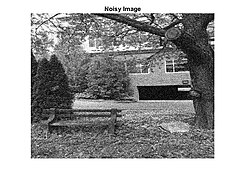
Image with Gaussian dissonance.

Prototype with Gaussian noise removed.

Wavelets are oftentimes used to denoise two dimensional signals, such every bit images. The following example provides three steps to remove unwanted white Gaussian racket from the noisy paradigm shown. Matlab was used to import and filter the epitome.

The start step is to choose a wavelet type, and a level North of decomposition. In this case biorthogonal 3.5 wavelets were chosen with a level N of 10. Biorthogonal wavelets are unremarkably used in prototype processing to detect and filter white Gaussian noise,^[21] due to their high contrast of neighboring pixel intensity values. Using these wavelets a wavelet transformation is performed on the two dimensional paradigm.

Post-obit the decomposition of the image file, the next step is to make up one's mind threshold values for each level from 1 to Northward. Birgé-Massart strategy^[22] is a fairly mutual method for selecting these thresholds. Using this process individual thresholds are made for N = 10 levels. Applying these thresholds are the majority of the actual filtering of the signal.

The final step is to reconstruct the paradigm from the modified levels. This is accomplished using an inverse wavelet transform. The resulting image, with white Gaussian racket removed is shown below the original paradigm. When filtering any form of data information technology is important to quantify the betoken-to-racket-ratio of the result.^{[ commendation needed ]} In this case, the SNR of the noisy image in comparison to the original was 30.4958%, and the SNR of the denoised image is 32.5525%. The resulting improvement of the wavelet filtering is a SNR gain of ii.0567%.^[23]

It is important to annotation that choosing other wavelets, levels, and thresholding strategies can consequence in different types of filtering. In this case, white Gaussian noise was chosen to be removed. Although, with dissimilar thresholding, it could just as hands have been amplified.

To illustrate the differences and similarities between the discrete wavelet transform with the discrete Fourier transform, consider the DWT and DFT of the following sequence: (one,0,0,0), a unit impulse.

The DFT has orthogonal ground (DFT matrix):

${\displaystyle {\begin{bmatrix}ane&ane&1&1\\one&-i&-1&i\\one&-1&ane&-ane\\1&i&-1&-i\end{bmatrix}}}$

while the DWT with Haar wavelets for length iv information has orthogonal footing in the rows of:

${\displaystyle {\begin{bmatrix}1&one&one&i\\1&1&-i&-ane\\1&-i&0&0\\0&0&1&-i\finish{bmatrix}}}$

(To simplify notation, whole numbers are used, then the bases are orthogonal just not orthonormal.)

Preliminary observations include:

• Sinusoidal waves differ merely in their frequency. The get-go does not consummate any cycles, the 2d completes one full wheel, the third completes two cycles, and the 4th completes three cycles (which is equivalent to completing one cycle in the reverse management). Differences in phase tin can exist represented by multiplying a given basis vector by a complex constant.
• Wavelets, by contrast, have both frequency and location. As before, the showtime completes goose egg cycles, and the 2nd completes one cycle. However, the third and quaternary both have the same frequency, twice that of the first. Rather than differing in frequency, they differ in location — the third is nonzero over the showtime ii elements, and the fourth is nonzero over the second two elements.

${\displaystyle {\brainstorm{aligned}(1,0,0,0)&={\frac {1}{4}}(1,1,1,1)+{\frac {one}{4}}(1,1,-i,-1)+{\frac {1}{ii}}(1,-1,0,0)\qquad {\text{Haar DWT}}\\(1,0,0,0)&={\frac {1}{four}}(i,1,1,1)+{\frac {one}{iv}}(1,i,-1,-i)+{\frac {1}{four}}(1,-1,1,-1)+{\frac {1}{4}}(1,-i,-1,i)\qquad {\text{DFT}}\end{aligned}}}$

The DWT demonstrates the localization: the (ane,1,1,1) term gives the average point value, the (ane,1,–1,–1) places the signal in the left side of the domain, and the (1,–1,0,0) places it at the left side of the left side, and truncating at whatsoever phase yields a downsampled version of the signal:

${\displaystyle {\begin{aligned}&\left({\frac {1}{4}},{\frac {1}{4}},{\frac {i}{4}},{\frac {1}{4}}\correct)\\&\left({\frac {1}{2}},{\frac {ane}{2}},0,0\correct)\qquad {\text{2-term truncation}}\\&\left(ane,0,0,0\right)\end{aligned}}}$

The DFT, by contrast, expresses the sequence by the interference of waves of various frequencies – thus truncating the serial yields a low-pass filtered version of the series:

${\displaystyle {\begin{aligned}&\left({\frac {one}{4}},{\frac {one}{iv}},{\frac {1}{4}},{\frac {1}{4}}\right)\\&\left({\frac {3}{4}},{\frac {i}{4}},-{\frac {1}{iv}},{\frac {1}{4}}\right)\qquad {\text{ii-term truncation}}\\&\left(one,0,0,0\correct)\end{aligned}}}$

Notably, the centre approximation (2-term) differs. From the frequency domain perspective, this is a better approximation, but from the time domain perspective it has drawbacks – information technology exhibits undershoot – one of the values is negative, though the original series is non-negative everywhere – and ringing, where the right side is non-zero, dissimilar in the wavelet transform. On the other hand, the Fourier approximation correctly shows a pinnacle, and all points are within ${\displaystyle 1/4}$ of their correct value, though all points accept fault. The wavelet approximation, by contrast, places a summit on the left half, but has no summit at the first betoken, and while it is exactly right for half the values (reflecting location), it has an error of ${\displaystyle 1/2}$ for the other values.

This illustrates the kinds of trade-offs between these transforms, and how in some respects the DWT provides preferable behavior, specially for the modeling of transients.

Definition [edit]

I level of the transform [edit]

The DWT of a bespeak ${\displaystyle ten}$ is calculated past passing it through a serial of filters. Start the samples are passed through a depression pass filter with impulse response ${\displaystyle g}$ resulting in a convolution of the ii:

${\displaystyle y[n]=(x*g)[due north]=\sum \limits _{yard=-\infty }^{\infty }{x[thousand]g[n-k]}}$

The signal is also decomposed simultaneously using a loftier-pass filter ${\displaystyle h}$ . The outputs give the particular coefficients (from the loftier-pass filter) and approximation coefficients (from the low-pass). It is important that the ii filters are related to each other and they are known every bit a quadrature mirror filter.

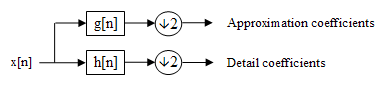
Block diagram of filter assay

All the same, since half the frequencies of the signal have now been removed, half the samples can be discarded according to Nyquist's dominion. The filter output of the low-pass filter ${\displaystyle g}$ in the diagram to a higher place is then subsampled past 2 and further candy by passing it again through a new low- pass filter ${\displaystyle g}$ and a loftier- laissez passer filter ${\displaystyle h}$ with one-half the cut-off frequency of the previous 1,i.e.:

${\displaystyle y_{\mathrm {low} }[n]=\sum \limits _{k=-\infty }^{\infty }{x[k]g[2n-one thousand]}}$

${\displaystyle y_{\mathrm {high} }[n]=\sum \limits _{m=-\infty }^{\infty }{x[1000]h[2n-1000]}}$

This decomposition has halved the fourth dimension resolution since only half of each filter output characterises the signal. However, each output has half the frequency ring of the input, then the frequency resolution has been doubled.

With the subsampling operator ${\displaystyle \downarrow }$

${\displaystyle (y\downarrow k)[due north]=y[kn]}$

the above summation tin can be written more concisely.

${\displaystyle y_{\mathrm {low} }=(x*g)\downarrow 2}$

${\displaystyle y_{\mathrm {high} }=(ten*h)\downarrow 2}$

However computing a consummate convolution ${\displaystyle x*k}$ with subsequent downsampling would waste matter computation time.

The Lifting scheme is an optimization where these two computations are interleaved.

Cascading and filter banks [edit]

This decomposition is repeated to further increase the frequency resolution and the approximation coefficients decomposed with loftier and low pass filters and and so downwards-sampled. This is represented as a binary tree with nodes representing a sub-infinite with a dissimilar fourth dimension-frequency localisation. The tree is known as a filter bank.

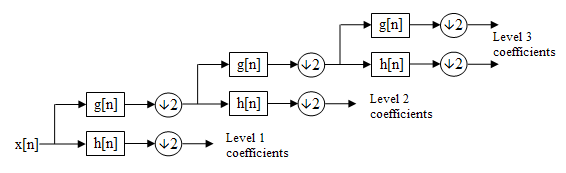
A 3 level filter banking company

At each level in the in a higher place diagram the signal is decomposed into low and loftier frequencies. Due to the decomposition process the input point must be a multiple of ${\displaystyle two^{north}}$ where ${\displaystyle n}$ is the number of levels.

For example a indicate with 32 samples, frequency range 0 to ${\displaystyle f_{n}}$ and 3 levels of decomposition, 4 output scales are produced:

Level	Frequencies	Samples
3	${\displaystyle 0}$ to ${\displaystyle {f_{n}}/eight}$	iv
	${\displaystyle {f_{n}}/8}$ to ${\displaystyle {f_{n}}/4}$	4
2	${\displaystyle {f_{due north}}/4}$ to ${\displaystyle {f_{n}}/2}$	8
1	${\displaystyle {f_{n}}/2}$ to ${\displaystyle f_{n}}$	16

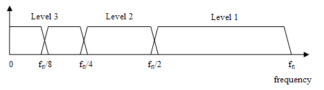
Frequency domain representation of the DWT

Relationship to the mother wavelet [edit]

The filterbank implementation of wavelets can be interpreted as calculating the wavelet coefficients of a detached set of child wavelets for a given mother wavelet ${\displaystyle \psi (t)}$ . In the instance of the discrete wavelet transform, the female parent wavelet is shifted and scaled past powers of 2

${\displaystyle \psi _{j,k}(t)={\frac {ane}{\sqrt {2^{j}}}}\psi \left({\frac {t-k2^{j}}{2^{j}}}\right)}$

where ${\displaystyle j}$ is the calibration parameter and ${\displaystyle k}$ is the shift parameter, both which are integers.

Call back that the wavelet coefficient ${\displaystyle \gamma }$ of a signal ${\displaystyle x(t)}$ is the projection of ${\displaystyle x(t)}$ onto a wavelet, and let ${\displaystyle x(t)}$ exist a signal of length ${\displaystyle 2^{N}}$ . In the instance of a child wavelet in the discrete family above,

${\displaystyle \gamma _{jk}=\int _{-\infty }^{\infty }x(t){\frac {ane}{\sqrt {2^{j}}}}\psi \left({\frac {t-k2^{j}}{2^{j}}}\correct)dt}$

Now fix ${\displaystyle j}$ at a particular scale, then that ${\displaystyle \gamma _{jk}}$ is a part of ${\displaystyle k}$ only. In light of the above equation, ${\displaystyle \gamma _{jk}}$ tin can be viewed every bit a convolution of ${\displaystyle x(t)}$ with a dilated, reflected, and normalized version of the female parent wavelet, ${\displaystyle h(t)={\frac {one}{\sqrt {two^{j}}}}\psi \left({\frac {-t}{2^{j}}}\right)}$ , sampled at the points ${\displaystyle 1,2^{j},2^{2j},...,2^{Northward}}$ . But this is precisely what the detail coefficients give at level ${\displaystyle j}$ of the discrete wavelet transform. Therefore, for an appropriate choice of ${\displaystyle h[n]}$ and ${\displaystyle g[n]}$ , the detail coefficients of the filter depository financial institution correspond exactly to a wavelet coefficient of a discrete set of kid wavelets for a given mother wavelet ${\displaystyle \psi (t)}$ .

As an example, consider the discrete Haar wavelet, whose mother wavelet is ${\displaystyle \psi =[ane,-ane]}$ . Then the dilated, reflected, and normalized version of this wavelet is ${\displaystyle h[n]={\frac {one}{\sqrt {two}}}[-1,1]}$ , which is, indeed, the highpass decomposition filter for the discrete Haar wavelet transform.

Time complexity [edit]

The filterbank implementation of the Detached Wavelet Transform takes only O(N) in sure cases, equally compared to O(Northward logNorth) for the fast Fourier transform.

Note that if ${\displaystyle k[n]}$ and ${\displaystyle h[n]}$ are both a constant length (i.east. their length is independent of N), then ${\displaystyle x*h}$ and ${\displaystyle 10*thousand}$ each take O(N) fourth dimension. The wavelet filterbank does each of these two O(N) convolutions, and so splits the point into 2 branches of size N/2. But it simply recursively splits the upper branch convolved with ${\displaystyle g[n]}$ (as assorted with the FFT, which recursively splits both the upper branch and the lower co-operative). This leads to the following recurrence relation

${\displaystyle T(North)=2N+T\left({\frac {N}{ii}}\right)}$

which leads to an O(North) time for the entire functioning, as can be shown by a geometric series expansion of the to a higher place relation.

Equally an example, the discrete Haar wavelet transform is linear, since in that case ${\displaystyle h[n]}$ and ${\displaystyle g[due north]}$ are constant length 2.

${\displaystyle h[n]=\left[{\frac {-{\sqrt {2}}}{two}},{\frac {\sqrt {2}}{2}}\right]thousand[northward]=\left[{\frac {\sqrt {2}}{2}},{\frac {\sqrt {2}}{2}}\right]}$

The locality of wavelets, coupled with the O(Northward) complexity, guarantees that the transform can exist computed online (on a streaming basis). This property is in sharp dissimilarity to FFT, which requires admission to the entire signal at one time. Information technology also applies to the multi-calibration transform and as well to the multi-dimensional transforms (east.thousand., two-D DWT).^[24]

Other transforms [edit]

• The Adam7 algorithm, used for interlacing in the Portable Network Graphics (PNG) format, is a multiscale model of the information which is similar to a DWT with Haar wavelets. Dissimilar the DWT, it has a specific calibration – information technology starts from an 8×8 block, and it downsamples the image, rather than decimating (depression-pass filtering, then downsampling). It thus offers worse frequency behavior, showing artifacts (pixelation) at the early stages, in render for simpler implementation.
• The multiplicative (or geometric) discrete wavelet transform ^[25] is a variant that applies to an observation model ${\displaystyle {\bf {y}}=f{\bf {X}}}$ involving interactions of a positive regular function ${\displaystyle f}$ and a multiplicative independent positive dissonance ${\displaystyle 10}$ , with ${\displaystyle \mathbb {East} Ten=ane}$ . Announce ${\displaystyle {\cal {W}}}$ , a wavelet transform. Since ${\displaystyle f{\bf {X}}=f+{f({\bf {10}}-ane)}}$ , then the standard (additive) discrete wavelet transform ${\displaystyle {\cal {W^{+}}}}$ is such that ${\displaystyle {\cal {W^{+}}}{\bf {y}}={\cal {Westward^{+}}}f+{\cal {W^{+}}}{f({\bf {X}}-i)},}$ where detail coefficients ${\displaystyle {\cal {W^{+}}}{f({\bf {X}}-1)}}$ cannot exist considered as thin in general, due to the contribution of ${\displaystyle f}$ in the latter expression. In the multiplicative framework, the wavelet transform is such that ${\displaystyle {\cal {W^{\times }}}{\bf {y}}=\left({\cal {Westward^{\times }}}f\correct)\times \left({\cal {W^{\times }}}{\bf {10}}\right).}$ This `embedding' of wavelets in a multiplicative algebra involves generalized multiplicative approximations and detail operators: For instance, in the instance of the Haar wavelets, so up to the normalization coefficient ${\displaystyle \alpha }$ , the standard ${\displaystyle {\cal {W^{+}}}}$ approximations (arithmetic mean) ${\displaystyle c_{k}=\alpha (y_{grand}+y_{m-1})}$ and details (arithmetic differences) ${\displaystyle d_{thou}=\alpha (y_{k}-y_{k-1})}$ become respectively geometric hateful approximations ${\displaystyle c_{k}^{\ast }=(y_{k}\times y_{g-1})^{\alpha }}$ and geometric differences (details) ${\displaystyle d_{k}^{\ast }=\left({\frac {y_{m}}{y_{k-1}}}\correct)^{\alpha }}$ when using ${\displaystyle {\cal {W^{\times }}}}$ .

Code example [edit]

In its simplest grade, the DWT is remarkably easy to compute.

The Haar wavelet in Java:

                        public            static            int            []            discreteHaarWaveletTransform            (            int            []            input            )            {            // This function assumes that input.length=two^north, northward>1            int            []            output            =            new            int            [            input            .            length            ]            ;            for            (            int            length            =            input            .            length            /            two            ;            ;            length            =            length            /            2            )            {            // length is the current length of the working area of the output array.            // length starts at one-half of the array size and every iteration is halved until it is 1.            for            (            int            i            =            0            ;            i            <            length            ;            ++            i            )            {            int            sum            =            input            [            i            *            ii            ]            +            input            [            i            *            2            +            1            ]            ;            int            difference            =            input            [            i            *            2            ]            -            input            [            i            *            ii            +            1            ]            ;            output            [            i            ]            =            sum            ;            output            [            length            +            i            ]            =            difference            ;            }            if            (            length            ==            1            )            {            return            output            ;            }            //Swap arrays to exercise next iteration            System            .            arraycopy            (            output            ,            0            ,            input            ,            0            ,            length            );            }            }          

Complete Java code for a 1-D and two-D DWT using Haar, Daubechies, Coiflet, and Legendre wavelets is available from the open source projection: JWave. Furthermore, a fast lifting implementation of the detached biorthogonal CDF 9/7 wavelet transform in C, used in the JPEG 2000 image compression standard tin can be found hither (archived 5 March 2012).

Example of in a higher place lawmaking [edit]

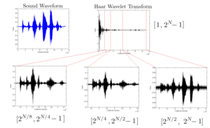
An case of computing the detached Haar wavelet coefficients for a sound point of someone saying "I Honey Wavelets." The original waveform is shown in bluish in the upper left, and the wavelet coefficients are shown in black in the upper correct. Along the lesser are shown three zoomed-in regions of the wavelet coefficients for different ranges.

This figure shows an instance of applying the above code to compute the Haar wavelet coefficients on a sound waveform. This example highlights ii key properties of the wavelet transform:

• Natural signals often have some degree of smoothness, which makes them sparse in the wavelet domain. There are far fewer significant components in the wavelet domain in this example than in that location are in the time domain, and near of the significant components are towards the coarser coefficients on the left. Hence, natural signals are compressible in the wavelet domain.
• The wavelet transform is a multiresolution, bandpass representation of a signal. This can be seen straight from the filterbank definition of the detached wavelet transform given in this article. For a bespeak of length ${\displaystyle 2^{N}}$ , the coefficients in the range ${\displaystyle [two^{North-j},2^{N-j+1}]}$ correspond a version of the original point which is in the pass-band ${\displaystyle \left[{\frac {\pi }{2^{j}}},{\frac {\pi }{2^{j-1}}}\right]}$ . This is why zooming in on these ranges of the wavelet coefficients looks so like in structure to the original signal. Ranges which are closer to the left (larger ${\displaystyle j}$ in the above notation), are coarser representations of the signal, while ranges to the right represent finer details.

Come across also [edit]

• Discrete cosine transform (DCT)
• Wavelet
• Wavelet series
• Wavelet pinch
• Listing of wavelet-related transforms

References [edit]

1. ^ A.N. Akansu, R.A. Haddad and H. Caglar, Perfect Reconstruction Binomial QMF-Wavelet Transform, Proc. SPIE Visual Communications and Prototype Processing, pp. 609–618, vol. 1360, Lausanne, Sept. 1990.
2. ^ Akansu, Ali N.; Haddad, Richard A. (1992), Multiresolution point decomposition: transforms, subbands, and wavelets, Boston, MA: Academic Press, ISBN 978-0-12-047141-6
3. ^ A.Northward. Akansu, Filter Banks and Wavelets in Signal Processing: A Disquisitional Review, Proc. SPIE Video Communications and PACS for Medical Applications (Invited Paper), pp. 330-341, vol. 1977, Berlin, Oct. 1993.
4. ^ Selesnick, I.W.; Baraniuk, R.G.; Kingsbury, North.C., 2005, The dual-tree circuitous wavelet transform
5. ^ Sullivan, Gary (8–12 December 2003). "Full general characteristics and design considerations for temporal subband video coding". ITU-T. Video Coding Experts Group. Retrieved thirteen September 2019.
6. ^ Bovik, Alan C. (2009). The Essential Guide to Video Processing. Bookish Press. p. 355. ISBN9780080922508.
7. ^ Gall, Didier Le; Tabatabai, Ali J. (1988). "Sub-band coding of digital images using symmetric brusque kernel filters and arithmetics coding techniques". ICASSP-88., International Conference on Acoustics, Speech, and Signal Processing: 761–764 vol.two. doi:10.1109/ICASSP.1988.196696. S2CID 109186495.
8. ^ Ali Naci Akansu, An Efficient QMF-Wavelet Structure (Binomial-QMF Daubechies Wavelets), Proc. 1st NJIT Symposium on Wavelets, April 1990.
9. ^ Said, A.; Pearlman, W. A. (1996). "A new, fast, and efficient image codec based on set up partitioning in hierarchical trees". IEEE Transactions on Circuits and Systems for Video Technology. half dozen (three): 243–250. doi:10.1109/76.499834. ISSN 1051-8215. Retrieved xviii Oct 2019.
10. ^ S. Mallat, A Wavelet Tour of Signal Processing, 2d ed. San Diego, CA: Academic, 1999.
11. ^ S. G. Mallat and S. Zhong, "Characterization of signals from multiscale edges," IEEE Trans. Design Anal. Mach. Intell., vol. 14, no. seven, pp. 710– 732, Jul. 1992.
12. ^ Ince, Kiranyaz, Gabbouj, 2009, A generic and robust organization for automated patient-specific classification of ECG signals
13. ^ "Novel method for stride length estimation with body area network accelerometers", IEEE BioWireless 2011, pp. 79–82
14. ^ Nasir, V.; Cool, J.; Sassani, F. (Oct 2019). "Intelligent Machining Monitoring Using Sound Signal Candy With the Wavelet Method and a Self-Organizing Neural Network". IEEE Robotics and Automation Letters. 4 (4): 3449–3456. doi:10.1109/LRA.2019.2926666. ISSN 2377-3766. S2CID 198474004.
15. ^ Broughton, S. Allen. "Wavelet Based Methods in Image Processing". www.rose-hulman.edu . Retrieved 2017-05-02 .
16. ^ Chervyakov, N. I.; Lyakhov, P. A.; Nagornov, N. N. (2018-xi-01). "Quantization Noise of Multilevel Discrete Wavelet Transform Filters in Image Processing". Optoelectronics, Instrumentation and Data Processing. 54 (6): 608–616. Bibcode:2018OIDP...54..608C. doi:10.3103/S8756699018060092. ISSN 1934-7944. S2CID 128173262.
17. ^ A.N. Akansu and M.J.T. Smith,Subband and Wavelet Transforms: Design and Applications, Kluwer Academic Publishers, 1995.
18. ^ A.Due north. Akansu and Thousand.J. Medley, Wavelet, Subband and Cake Transforms in Communications and Multimedia, Kluwer Academic Publishers, 1999.
19. ^ A.N. Akansu, P. Duhamel, 10. Lin and Grand. de Courville Orthogonal Transmultiplexers in Communication: A Review, IEEE Trans. On Betoken Processing, Special Outcome on Theory and Applications of Filter Banks and Wavelets. Vol. 46, No.four, pp. 979–995, April, 1998.
20. ^ A.Northward. Akansu, W.A. Serdijn, and I.W. Selesnick, Wavelet Transforms in Signal Processing: A Review of Emerging Applications, Concrete Communication, Elsevier, vol. 3, issue ane, pp. 1–18, March 2010.
21. ^ Pragada, S.; Sivaswamy, J. (2008-12-01). "Image Denoising Using Matched Biorthogonal Wavelets". 2008 6th Indian Briefing on Calculator Vision, Graphics Image Processing: 25–32. doi:10.1109/ICVGIP.2008.95. S2CID 15516486.
22. ^ "Thresholds for wavelet one-D using Birgé-Massart strategy - MATLAB wdcbm". world wide web.mathworks.com . Retrieved 2017-05-03 .
23. ^ "how to become SNR for 2 images - MATLAB Answers - MATLAB Central". www.mathworks.com . Retrieved 2017-05-x .
24. ^ Barina, David (2020). "Real-time wavelet transform for space image strips". Journal of Real-Fourth dimension Image Processing. Springer. 18 (iii): 585–591. doi:10.1007/s11554-020-00995-8. S2CID 220396648. Retrieved 2020-07-09 .
25. ^ Atto, Abdourrahmane M.; Trouvé, Emmanuel; Nicolas, Jean-Marie; Lê, Thu Trang (2016). "Wavelet Operators and Multiplicative Observation Models—Application to SAR Image Fourth dimension-Series Analysis" (PDF). IEEE Transactions on Geoscience and Remote Sensing. 54 (11): 6606–6624. Bibcode:2016ITGRS..54.6606A. doi:10.1109/TGRS.2016.2587626. S2CID 1860049.

^[1]

External links [edit]

• Stanford's WaveLab in matlab
• libdwt, a cross-platform DWT library written in C
• Concise Introduction to Wavelets by René Puschinger

1. ^ Prasad, Akhilesh; Maan, Jeetendrasingh; Verma, Sandeep Kumar (2021). "Wavelet transforms associated with the index Whittaker transform". Mathematical Methods in the Applied Sciences. 44 (13): 10734–10752. Bibcode:2021MMAS...4410734P. doi:10.1002/mma.7440. ISSN 1099-1476. S2CID 235556542.

How Are The Low And High Pass Filters For Dwt Chosen,

Source: https://en.wikipedia.org/wiki/Discrete_wavelet_transform

Posted by: bootsdoner1941.blogspot.com

Share this post